Eric Almeida, Kevin Luczak, Dasith Perera
RNA Sequencing is used to investigate the transcriptional profile of a cell
Genome (DNA) -> Transcriptome (RNA) -> Protein
RNA Transcripts are used to:
- transcribe proteins
- form the ribosomal translation machinery
- regulate gene expression
- modulate proteins
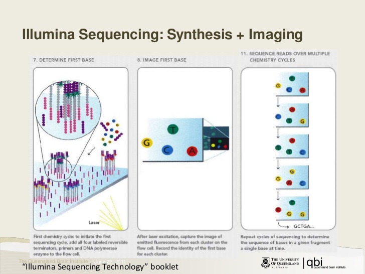
RNA can be sequenced using Next Generation Sequencing

? 2017 Illumina, Inc. All rights reserved.
Illumina sequencing-by-synthesis
Example RNA-sequencing workflow
- Step 1. Experimental Design
- Step 2. Library Preparation
- Step 3. Execute the experiment
- Step 4. Align sequencing data to reference genome using BowTie2
- Step 5. Obtain count data using htseq-count
- Step 6. Move data into R and generate results
NOISeq Install from Bioconductor
source("https://bioconductor.org/biocLite.R") #Downloading from Bioconductor
biocLite("NOISeq")
library(NOISeq)
Help Viewer in R
Documentation and help can be easily accessed through the “? (command)” command
In example:
-
?head # takes you to Help viewer for ‘head’ command
-
?noiseq # takes you to Help viewer for noiseq package
View Input Data
Load your data into R and make your own treatment groups
data(Marioni)
head(mycounts) #Count data (data from upstream)

##                 R1L1Kidney R1L2Liver R1L3Kidney R1L4Liver R1L6Liver
## ENSG00000177757          2         1          0         0         1
## ENSG00000187634         49        27         43        34        23
## ENSG00000188976         73        34         77        56        45
## ENSG00000187961         15         8         15        13        11
## ENSG00000187583          1         0          1         1         0
## ENSG00000187642          4         0          5         0         2
##                 R1L7Kidney R1L8Liver R2L2Kidney R2L3Liver R2L6Kidney
## ENSG00000177757          2         0          1         1          3
## ENSG00000187634         41        35         42        25         47
## ENSG00000188976         68        55         70        42         82
## ENSG00000187961         13        12         12        20         15
## ENSG00000187583          3         0          0         2          3
## ENSG00000187642         12         1          9         4          9

head(myfactors) #Treatment groups / replicates as you define it

##            Tissue TissueRun
## R1L1Kidney Kidney  Kidney_1
## R1L2Liver   Liver   Liver_1
## R1L3Kidney Kidney  Kidney_1
## R1L4Liver   Liver   Liver_1
## R1L6Liver   Liver   Liver_1
## R1L7Kidney Kidney  Kidney_1

myfactors = data.frame(Tissue = c("Kidney", "Liver", "Kidney", "Liver", "Liver", "Kidney", "Liver", "Kidney", "Liver", "Kidney"), TissueRun = c("Kidney_1", "Liver_1", "Kidney_1", "Liver_1", "Liver_1", "Kidney_1", "Liver_1",  "Kidney_2", "Liver_2", "Kidney_2"), Run = c(rep("R1", 7), rep("R2", 3)))
myfactors #Should see the other defined treatment groups

##    Tissue TissueRun Run
## 1  Kidney  Kidney_1  R1
## 2   Liver   Liver_1  R1
## 3  Kidney  Kidney_1  R1
## 4   Liver   Liver_1  R1
## 5   Liver   Liver_1  R1
## 6  Kidney  Kidney_1  R1
## 7   Liver   Liver_1  R1
## 8  Kidney  Kidney_2  R2
## 9   Liver   Liver_2  R2
## 10 Kidney  Kidney_2  R2
Additional Bioinformation, from Ensembl Biomart
Provided for us in the Marioni data set, but easy to DIY. In example, first download the unique gene ID and biotype to a csv file from an online database that contains this information on your organism of study, then:
#GENES <- read.csv("C:/Users/labuser/Documents/R/GENES.txt")
#GENES1 <- data.frame(GENES$'Gene.stable.ID')
#GENES1$Gene.Type <- GENES$'Gene.type'
#GENES2 <- unique(GENES1)
#ID <- GENES2$'GENES.Gene.stable.ID'
#TYPE <- GENES2$'Gene.Type'
#BIOTYPES <- data.frame(TYPE)
#row.names(BIOTYPES) <- GENES2$'GENES.Gene.stable.ID'
Creating a NOISeq Object
mydata <- readData(data = mycounts, length = mylength, gc = mygc, biotype = mybiotypes, chromosome = mychroms, factors = myfactors)
mydata

## ExpressionSet (storageMode: lockedEnvironment)
## assayData: 5088 features, 10 samples
##   element names: exprs
## protocolData: none
## phenoData
##   sampleNames: R1L1Kidney R1L2Liver ... R2L6Kidney (10 total)
##   varLabels: Tissue TissueRun Run
##   varMetadata: labelDescription
## featureData
##   featureNames: ENSG00000177757 ENSG00000187634 ...
##     ENSG00000201145 (5088 total)
##   fvarLabels: Length GC ... GeneEnd (6 total)
##   fvarMetadata: labelDescription
## experimentData: use 'experimentData(object)'
## Annotation:
QC Plots
Biases (error) are introduced through RNA extraction, library preparation, and sequencing processes
Quality control tests offered by NOISeq:
- Biotype detection
- QC Bias
- Length Bias
- RNA composition
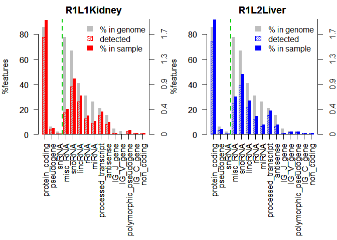
Biotype Detection
- Used to quickly visualize potential contamination or technical biases introduced during library preparation
mybiodetection <- dat(mydata, k=0, type = "biodetection", factor = NULL)

## Biotypes detection is to be computed for:
##  [1] "R1L1Kidney" "R1L2Liver"  "R1L3Kidney" "R1L4Liver"  "R1L6Liver"
##  [6] "R1L7Kidney" "R1L8Liver"  "R2L2Kidney" "R2L3Liver"  "R2L6Kidney"

par(mfrow = c(1,2))
explo.plot(mybiodetection, samples = c(1,2), plottype ="persample")
Biotype Detection, output 2
mybiodetection <- dat(mydata, k=0, type = "biodetection", factor = NULL)

## Biotypes detection is to be computed for:
##  [1] "R1L1Kidney" "R1L2Liver"  "R1L3Kidney" "R1L4Liver"  "R1L6Liver"
##  [6] "R1L7Kidney" "R1L8Liver"  "R2L2Kidney" "R2L3Liver"  "R2L6Kidney"

par(mfrow = c(1,2))
explo.plot(mybiodetection, samples = c(1,2), toplot = "protein_coding", plottype ="comparison")
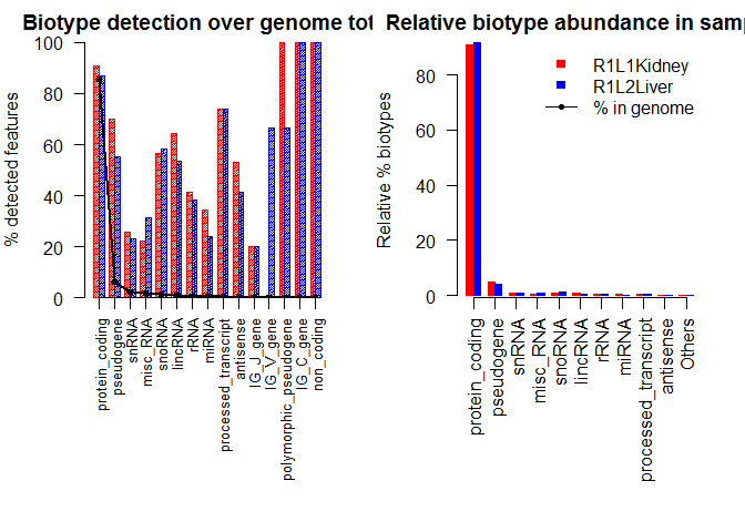
## [1] "Percentage of protein_coding biotype in each sample:"
## R1L1Kidney  R1L2Liver
##    91.0181    91.7060
## [1] "Confidence interval at 95% for the difference of percentages: R1L1Kidney - R1L2Liver"
## [1] -1.7991  0.4233
## [1] "The percentage of this biotype is NOT significantly different for these two samples (p-value = 0.2302 )."
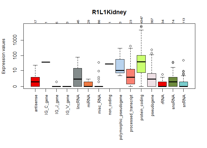
Biotype Detection, output 3
mycountsbio <- dat(mydata, factor = NULL, type = "countsbio")

## [1] "Count distributions are to be computed for:"
##  [1] "R1L1Kidney" "R1L2Liver"  "R1L3Kidney" "R1L4Liver"  "R1L6Liver"
##  [6] "R1L7Kidney" "R1L8Liver"  "R2L2Kidney" "R2L3Liver"  "R2L6Kidney"

explo.plot(mycountsbio, toplot = 1, samples = 1, plottype ="boxplot")
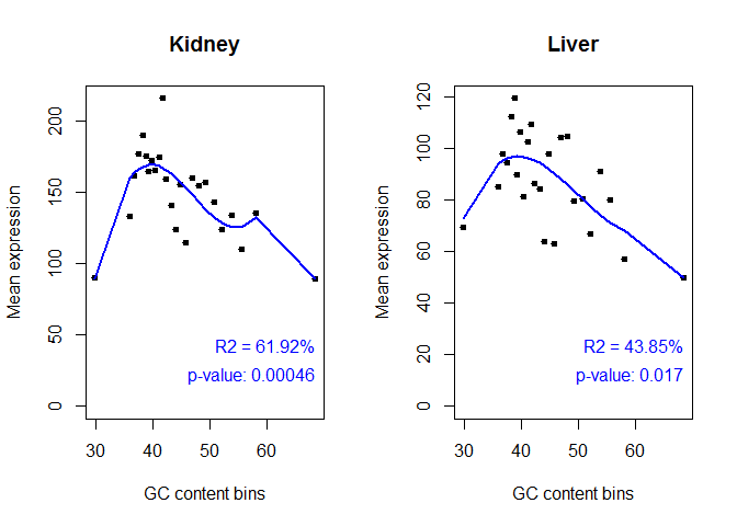
GC Bias
- Used to gauge whether sequencing bias has favored transcripts with low GC content
myGCbias = dat(mydata, factor = "Tissue", type = "GCbias")

## [1] "GC content bias detection is to be computed for:"
## [1] "Kidney" "Liver"
## [1] "Kidney"
##
## Call:
## lm(formula = datos[, i] ~ bx)
##
## Residuals:
##     Min      1Q  Median      3Q     Max
## -38.136  -4.568   0.832  10.406  48.852
##
## Coefficients: (1 not defined because of singularities)
##             Estimate Std. Error t value Pr(>|t|)
## (Intercept)  89.4686    20.2643   4.415 0.000267 ***
## bx1           0.2447    28.1216   0.009 0.993144
## bx2         177.5119    36.0617   4.922 8.22e-05 ***
## bx3         -68.5025    57.1321  -1.199 0.244534
## bx4         107.6385    64.0141   1.681 0.108220
## bx5               NA         NA      NA       NA
## ---
## Signif. codes:  0 '***' 0.001 '**' 0.01 '*' 0.05 '.' 0.1 ' ' 1
##
## Residual standard error: 20.26 on 20 degrees of freedom
## Multiple R-squared:  0.6192, Adjusted R-squared:  0.543
## F-statistic:  8.13 on 4 and 20 DF,  p-value: 0.0004613
##
## [1] "Liver"
##
## Call:
## lm(formula = datos[, i] ~ bx)
##
## Residuals:
##     Min      1Q  Median      3Q     Max
## -29.424  -9.185   0.000   9.384  22.594
##
## Coefficients: (1 not defined because of singularities)
##             Estimate Std. Error t value Pr(>|t|)
## (Intercept)   49.862     15.000   3.324  0.00338 **
## bx1           22.700     20.816   1.091  0.28845
## bx2           75.753     26.694   2.838  0.01017 *
## bx3            7.595     42.291   0.180  0.85927
## bx4           18.511     47.385   0.391  0.70019
## bx5               NA         NA      NA       NA
## ---
## Signif. codes:  0 '***' 0.001 '**' 0.01 '*' 0.05 '.' 0.1 ' ' 1
##
## Residual standard error: 15 on 20 degrees of freedom
## Multiple R-squared:  0.4385, Adjusted R-squared:  0.3262
## F-statistic: 3.904 on 4 and 20 DF,  p-value: 0.01678

explo.plot(myGCbias, samples = NULL, toplot = "global")
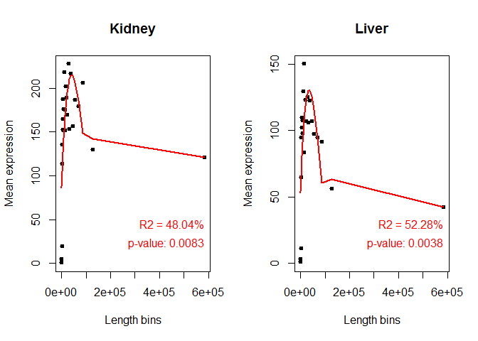
Length Bias
- Used to elucidate if bias is brought about by gene length
mylengthbias = dat(mydata, factor = "Tissue", type = "lengthbias")

## [1] "Length bias detection information is to be computed for:"
## [1] "Kidney" "Liver"
## [1] "Kidney"
##
## Call:
## lm(formula = datos[, i] ~ bx)
##
## Residuals:
##     Min      1Q  Median      3Q     Max
## -85.399 -19.603   3.049  25.848  74.827
##
## Coefficients: (1 not defined because of singularities)
##             Estimate Std. Error t value Pr(>|t|)
## (Intercept)   121.33      48.63   2.495  0.02148 *
## bx1           -34.97      52.24  -0.670  0.51082
## bx2           269.24      88.41   3.045  0.00639 **
## bx3         -1301.13     719.73  -1.808  0.08570 .
## bx4          6292.42    4655.39   1.352  0.19158
## bx5               NA         NA      NA       NA
## ---
## Signif. codes:  0 '***' 0.001 '**' 0.01 '*' 0.05 '.' 0.1 ' ' 1
##
## Residual standard error: 48.63 on 20 degrees of freedom
## Multiple R-squared:  0.4804, Adjusted R-squared:  0.3764
## F-statistic: 4.622 on 4 and 20 DF,  p-value: 0.008332
##
## [1] "Liver"
##
## Call:
## lm(formula = datos[, i] ~ bx)
##
## Residuals:
##    Min     1Q Median     3Q    Max
## -51.84 -18.19   0.00  21.29  42.30
##
## Coefficients: (1 not defined because of singularities)
##             Estimate Std. Error t value Pr(>|t|)
## (Intercept)    42.18      29.68   1.421 0.170729
## bx1            10.75      31.88   0.337 0.739524
## bx2           222.14      53.96   4.117 0.000535 ***
## bx3         -1141.68     439.26  -2.599 0.017161 *
## bx4          5758.12    2841.23   2.027 0.056243 .
## bx5               NA         NA      NA       NA
## ---
## Signif. codes:  0 '***' 0.001 '**' 0.01 '*' 0.05 '.' 0.1 ' ' 1
##
## Residual standard error: 29.68 on 20 degrees of freedom
## Multiple R-squared:  0.5228, Adjusted R-squared:  0.4273
## F-statistic: 5.477 on 4 and 20 DF,  p-value: 0.003815

explo.plot(mylengthbias, samples = NULL, toplot ="global")
Length Bias, output 2
show(mylengthbias)

## [1] "Kidney"
##
## Call:
## lm(formula = datos[, i] ~ bx)
##
## Residuals:
##     Min      1Q  Median      3Q     Max
## -85.399 -19.603   3.049  25.848  74.827
##
## Coefficients: (1 not defined because of singularities)
##             Estimate Std. Error t value Pr(>|t|)
## (Intercept)   121.33      48.63   2.495  0.02148 *
## bx1           -34.97      52.24  -0.670  0.51082
## bx2           269.24      88.41   3.045  0.00639 **
## bx3         -1301.13     719.73  -1.808  0.08570 .
## bx4          6292.42    4655.39   1.352  0.19158
## bx5               NA         NA      NA       NA
## ---
## Signif. codes:  0 '***' 0.001 '**' 0.01 '*' 0.05 '.' 0.1 ' ' 1
##
## Residual standard error: 48.63 on 20 degrees of freedom
## Multiple R-squared:  0.4804, Adjusted R-squared:  0.3764
## F-statistic: 4.622 on 4 and 20 DF,  p-value: 0.008332
##
## [1] "Liver"
##
## Call:
## lm(formula = datos[, i] ~ bx)
##
## Residuals:
##    Min     1Q Median     3Q    Max
## -51.84 -18.19   0.00  21.29  42.30
##
## Coefficients: (1 not defined because of singularities)
##             Estimate Std. Error t value Pr(>|t|)
## (Intercept)    42.18      29.68   1.421 0.170729
## bx1            10.75      31.88   0.337 0.739524
## bx2           222.14      53.96   4.117 0.000535 ***
## bx3         -1141.68     439.26  -2.599 0.017161 *
## bx4          5758.12    2841.23   2.027 0.056243 .
## bx5               NA         NA      NA       NA
## ---
## Signif. codes:  0 '***' 0.001 '**' 0.01 '*' 0.05 '.' 0.1 ' ' 1
##
## Residual standard error: 29.68 on 20 degrees of freedom
## Multiple R-squared:  0.5228, Adjusted R-squared:  0.4273
## F-statistic: 5.477 on 4 and 20 DF,  p-value: 0.003815
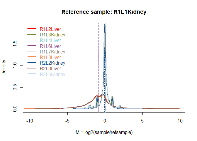
RNA composition
mycd = dat(mydata, type = "cd", norm = FALSE, refColumn = 1)

## [1] "Reference sample is: R1L1Kidney"
## [1] "Confidence intervals for median of M:"
##            0.28%                 99.72%                Diagnostic Test
## R1L2Liver  "-0.891798603865612"  "-0.766824549577716"  "FAILED"
## R1L3Kidney "-0.0471703644087826" "-0.0471703644087824" "FAILED"
## R1L4Liver  "-0.879624287764932"  "-0.7540048872931"    "FAILED"
## R1L6Liver  "-0.903134087665681"  "-0.761454067082924"  "FAILED"
## R1L7Kidney "0.0348451027997053"  "0.0348451027997056"  "FAILED"
## R1L8Liver  "-0.904500838561669"  "-0.760538326376263"  "FAILED"
## R2L2Kidney "-0.0850229820491386" "-0.0468824681954803" "FAILED"
## R2L3Liver  "-0.879935949269671"  "-0.749483184477486"  "FAILED"
## R2L6Kidney "-0.0726984636810064" "-0.0363901813919369" "FAILED"
## [1] "Diagnostic test: FAILED. Normalization is required to correct this bias."

explo.plot(mycd)
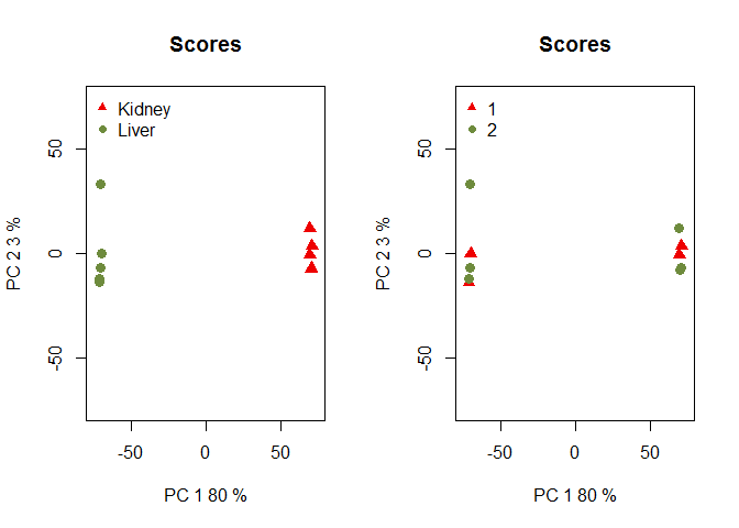
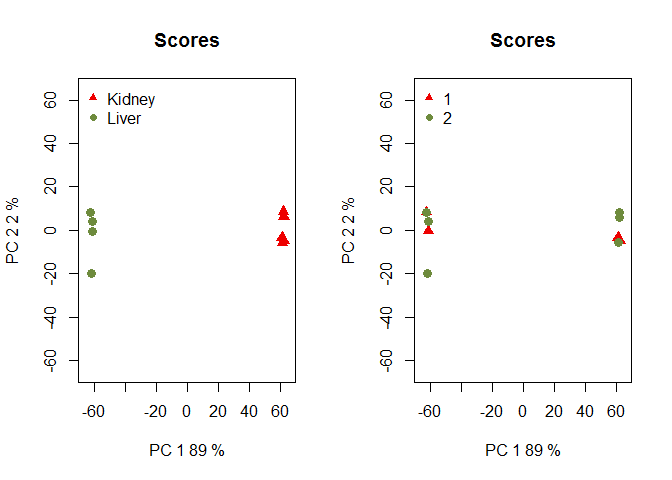
Batch effect
Here, we introduce a batch effect in example, and will later correct for it:
set.seed(123)
mycounts2 = mycounts
mycounts2[, 1:4] = mycounts2[, 1:4]
runif(nrow(mycounts2) * 4, 3, 5)
myfactors = data.frame(myfactors, batch = c(rep(1, 4), rep(2, 6)))
mydata2 = readData(mycounts2, factors = myfactors)
myPCA = dat(mydata2, type = "PCA")
par(mfrow = c(1, 2))
explo.plot(myPCA, factor = "Tissue")
explo.plot(myPCA, factor = "batch")
Sequencing Depth
A key question in RNA-Seq:
- Are the number of sequencing reads enough to study our genome and to properly quantify feature expression?
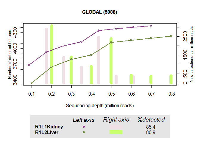
Saturation plot
-
How many features in the genome are being detected with more than a given number of counts, k (k=0 or k=5)
-
How the number of detected features would change with increasing sequencing depth
- For all features or for each biotype
Saturation plot
mysaturation = dat(mydata, k = 0, ndepth = 7, type = "saturation")
explo.plot(mysaturation, toplot = 1, samples = 1:2, yleftlim = NULL,
yrightlim = NULL)
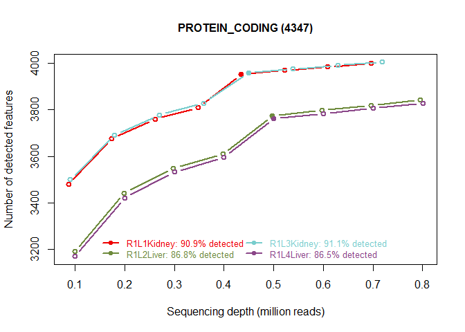
Distribution of protein-coding genes of a specific biotype
explo.plot(mysaturation, toplot="protein_coding", samples=1:4)
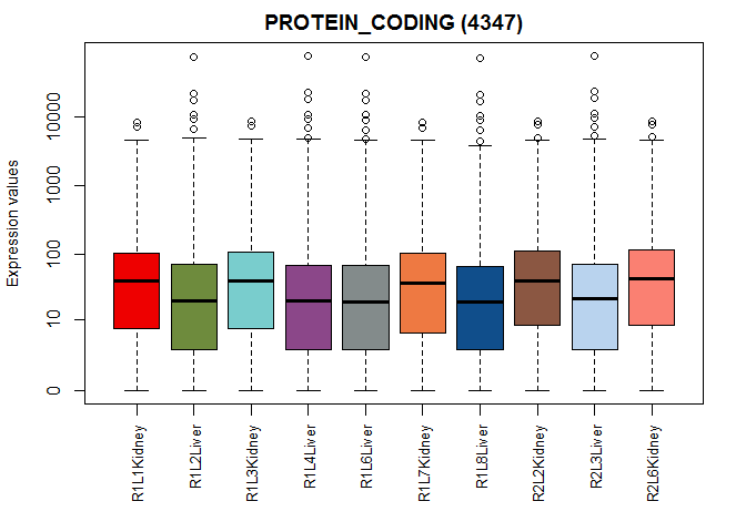
Count distribution for all samples for a certain biotype
explo.plot(mycountsbio, toplot = "protein_coding", samples = NULL,
plottype = "boxplot")
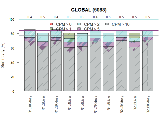
Sensitivity plot
explo.plot(mycountsbio, toplot = 1, samples = NULL, plottype = "barplot")
Filtering low counts
- Excluding low counts generally improves differential expression
results
- noise is reduced
- The best procedure to filter low count features is unknown
- NOISeq proposes 3 different methods to filter out features with low
counts:
- CPM Method
- Wilcoxon test
- Proportion test
myfilt = filtered.data(mycounts, factor = myfactors$Tissue, norm = FALSE,
depth = NULL, method = 1, cv.cutoff = 100, cpm = 1)

## Filtering out low count features...
## 4406 features are to be kept for differential expression analysis with filtering method 1
Normalization
- Necessary to analyze between samples and remove sequencing depth bias
- Can normalize in RPKM, Upper Quartile, and TMM
##                 R1L1Kidney  R1L2Liver R1L3Kidney  R1L4Liver  R1L6Liver
## ENSG00000177757   1.866057  0.8160788  0.0000000  0.0000000  0.8375346
## ENSG00000187634  22.597824 10.8910916 19.1928426 13.6356594  9.5215171
## ENSG00000188976  43.360221 17.6638209 44.2649178 28.9256646 23.9932411
## ENSG00000187961   6.946966  3.2406417  6.7235013  5.2356905  4.5730336
## ENSG00000187583   0.270246  0.0000000  0.2615529  0.2350098  0.0000000
## ENSG00000187642   1.334678  0.0000000  1.6146812  0.0000000  0.5990378
##                 R1L7Kidney R1L8Liver R2L2Kidney  R2L3Liver R2L6Kidney
## ENSG00000177757   1.911677  0.000000   0.879631  0.7854861  2.5794742
## ENSG00000187634  19.370633 14.972295  18.261034  9.7063073 19.9748412
## ENSG00000188976  41.377759 30.302685  39.198749 21.0020365 44.8846064
## ENSG00000187961   6.167891  5.155075   5.239510  7.7978955  6.4019183
## ENSG00000187583   0.830558  0.000000   0.000000  0.4550224  0.7471288
## ENSG00000187642   4.101920  0.309504   2.831161  1.1236213  2.7674127
Normalization Cheat Sheet
-
long = Numeric vector containing the length of the features
-
k, Counts equal to 0 are changed to k in order to avoid indeterminations when applying logarithms. By default, k = 0
-
k = NULL, makes all zero values into a value between 0 and the lowest non-zero value.
-
lc = Correction factor for length normalization. This correction is done by dividing the counts vector by (length/1000)lc. If lc = 0, no length correction is applied. By default, lc = 1 for RPKM and lc = 0 for the other methods.
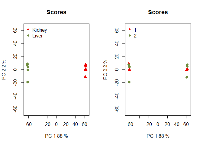
Batch Effect Correction
- ARSyNseq filters the noise associated to identified or not identified batch effects considering the experimental design and applying Principal Component Analysis (PCA) to the analysis of variance (ANOVA) parameters and residuals.
If the batch for each sample is known:
Batch is unknown
If the batch for each sample is unknown:
NOISeq options
-
Designed to compute differential expression on data:
- With technical replicates (NOISeq-real)
- No replicates at all! (NOISeq-sim)
-
NOISeq-real used when technical replicates are available.
- Summarizes by summing them up
-
NOISeq-real can be used on Biological replicates
- Averages replicates instead of summing.
- Manual recommends use of NOISeqBIO for biological replicates
How NOISeq-real works- Summarized
NOISeq-real estimates the probability distribution for M and D in an empirical way, by computing M and D values for every pair of replicates within the same experimental condition and for every feature. Then, all these values are pooled together to generate the noise distribution*
M = log2-ratio of the two conditions
D = the value of the difference between conditions.
A feature is differentially expressed if its corresponding M and D values are likely to be higher than in noise.
Disclaimer: Biological replicates are necessary if the goal is to make any inference about the population. Deriving differential expression from technical replicates is useful for drawing conclusions about the specific samples being compared in the study but not for extending these conclusions to the whole population
*When using NOISeq-real for biological values are averaged instead of summed up.
NOISeq-sim
NOISeq can simulate technical replicates
-
Assumes that read counts follow a multinomial distribution
-
probabilities for each feature in the multinomial distribution are the probablility of a read to map onto that feature.
-
mapping probability are approximated by using counts in the only sample of the corresponding experimental condition.
NOISeq-real & NOISeq-sim
NOISeq-real
mynoiseq = noiseq(mydata, k= 0.5, norm = "rpkm", factor = "Tissue", pnr = 0.2,
nss = 5, v = 0.02, lc = 1, replicates = "technical")

## [1] "Computing (M,D) values..."
## [1] "Computing probability of differential expression..."
NOISeq-sim
myresults <- noiseq(mydata, factor = "Tissue", k = NULL, norm = "n", pnr = 0.2,
nss = 5, v = 0.02, lc = 1, replicates = "no")

## [1] "Computing (M,D) values..."
## [1] "Computing probability of differential expression..."
NOISeqBIO
Optimized for use on biological replicates (at least 2 per condition).
Too much stats- see page 20 of NOISeq manual
mynoiseqbio = noiseqbio(mydata, k = 0.5, norm = "rpkm", factor = "Tissue",
lc = 1, r = 20, adj = 1.5, plot = FALSE, a0per = 0.9, random.seed = 12345,
filter = 2)

## Computing Z values...
## Filtering out low count features...
## 5088 features are to be kept for differential expression analysis with filtering method 2
## [1] "r = 1"
## [1] "r = 2"
## [1] "r = 3"
## [1] "r = 4"
## [1] "r = 5"
## [1] "r = 6"
## [1] "r = 7"
## [1] "r = 8"
## [1] "r = 9"
## [1] "r = 10"
## [1] "r = 11"
## [1] "r = 12"
## [1] "r = 13"
## [1] "r = 14"
## [1] "r = 15"
## [1] "r = 16"
## [1] "r = 17"
## [1] "r = 18"
## [1] "r = 19"
## [1] "r = 20"
## Computing probability of differential expression...
## p0 = 0.132948760535283
## Probability
##    Min. 1st Qu.  Median    Mean 3rd Qu.    Max.
##  0.0000  0.9049  0.9937  0.8680  1.0000  1.0000
Results
To look at the number of differentially expressed genes (DEGs):
Works-cited
##
##   Tarazona, S., Garcia-Alcalde, F., Dopazo, J., Ferrer, A., &
##   Conesa, A. (2011). Differential expression in RNA-seq: a matter
##   of depth. Genome Research, 21(12), 2213-2223.
##
##   Tarazona, S., Furio-Tari, P., Turra, D., Di Pietro, A., Nueda,
##   M.J., Ferrer, A., & Conesa, A. (2015). Data quality aware
##   analysis of differential expression in RNA-seq with NOISeq
##   R/Bioc package. Nucleic Acids Research.
Comments